- Product
- Solutions
Solutions
Unparalleled performance for organizations requiring maximum security, control and efficiencyTailored automated gating pipelines trained on your data, for your useStreamline your data journey with automated uploads, end-to-end traceability, and integrated analysis - Resources
- Support
- Pricing
- Sign In
Guide to flowAI in OMIQ
A guide covering flowAI in OMIQ, the algorithm for automated data cleaning.
Background
FCS data commonly has anomalies in it that can confound analysis. These anomalies can be caused by issues with the instrument, samples, and acquisition. Examples could include clogs, clumps, bumps, tube changes, etc. Given the potential to confound analysis, it is desired to have a way to automatically remove affected regions of data. flowAI is one such computational method for doing this. This guide discusses flowAI but also often generalizes to any cleaning algorithm.
Paper Reference
flowAI: automatic and interactive anomaly discerning tools for flow cytometry data. Gianni Monaco, Hao Chen, Michael Poidinger, Jinmiao Chen, João Pedro de Magalhães, Anis Larbi. 2016 Bioinformatics.
Algorithm Overview
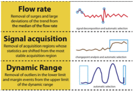
flowAI is an algorithm designed to automatically clean FCS data of undesired events. To accomplish this it looks at three different properties of the data using methods to find anomalies that should be discarded. The properties/methods are:
- Flow Rate (FR). With Flow Rate analysis, flowAI looks for significant deviations from the median flow rate of the file and identifies these regions for rejection.
- Signal Acquisition (FS). With Signal Acquisition analysis, flowAI looks at the signal in each channel over time. It establishes which contiguous time region has the most stable signal across all channels. This region is kept, while the rest of the data are rejected.
- Dynamic Range (FM). With Dynamic Range analysis, flowAI looks at all channels for negative and positive outlier events for rejection.
Notes:
- The two-letter abbreviations are part of the official flowAI package terminology.
- flowAI always examines all three properties of the data and includes this analysis in the report. However, which properties are used to actually clean the data are up to the user.
Example Data
This document uses these FCS files which were included with the flowAI package as example data. There are three files within the zip file and they are useful for trying out the algorithm.
Video Overview
► Watch the Automated Data Cleaning video series
Subsampling
The general purpose and behavior of the Subsampling Task in OMIQ should be known. If not, please consult the relevant section in the main documentation and understand its importance for normal algorithm runs.
A common question around data cleaning algorithms is if subsampling still serves the same purpose as it normally would when running other algorithms. In short, the answer is no, but there are important related details and exceptions to discuss.
The reason the short answer is no is because most algorithms require subsampling to feed in clean data to the algorithm (e.g., removing dead cells, doublets, debris, etc.) because most algorithms are meant to operate on clean data to produce a result used for scientific interpretation. You don’t want to confound the interpretation of that result with nonsensical cellular data. This same objective does not exist with cleaning algorithms. They are designed to aid in the process of preparing data for actual scientific analysis, not in producing a scientifically interpretable result on their own. Optional exceptions to this are discussed below, but note one unique exception of having beads mixed in with the sample data. As a general rule beads must be removed from the data prior to running a cleaning algorithm or a number of unusual behaviors or failures may result.
With the above being said, while it is not a requirement to provide clean data to a cleaning algorithm, it is neither wrong nor harmful to do so. It is an acceptable strategy. It can also be an optimization strategy for computational time or quality of cleaning results. Consider a scenario where a given file has a very large percentage of dead cells, debris, doublets, etc. If you know you will be removing these eventually, it can be more efficient to remove them ahead of time because it avoids the computational time that would otherwise be spent on these unwanted data. In extreme cases the “garbage” could be such a large fraction of the file that the distribution of signal over time is not representative and the cleaning algorithm operates sub-optimally. In these cases, it could be beneficial to preclean the data to allow the algorithm to focus on the remainder and hopefully improve the quality of the result.
Please note especially that using cleaning algorithms does not remove the requirement to also clean your data with traditional gate-based strategies (as noted above, either before or after). Cleaning algorithms identify anomalies in data distribution consistency over time. These types of anomalies are usually associated with problems with acquisition at the instrument level, such as clogs, bubbles, fluidics problems, etc. Cleaning algorithms do NOT identify issues with cellular data quality such as debris, doublets, dead cells, etc., which are irrelevant to signal over time and generally appear in consistent ratios through the acquisition. These unwanted data are generally filtered out through some specific gating strategy (such gating steps can be automated but that’s a different discussion). We do acknowledge that these two concepts can dovetail to some extent, such as some very large non-clogging clump of cells passing through the flow stream. This perhaps could be filtered out as an extreme doublet but also could appear as a time-based anomaly. The real test is not the means of origin of the anomaly, but whether it registers as an anomaly in signal over time. If yes, then the cleaning algorithm will target it. If not, then the anomaly would be left for other forms of cleanup.
Algorithm Settings and Setup
In this section, there are written descriptions of each flowAI setting. Remember that descriptions of how each method works are given in the Algorithm Overview section. These descriptions are useful to review when considering each setting.
Subsampling and Pre Filter
See the section above to understand the role of Subsampling in the application of cleaning algorithms.
If you determine that you want to subsample the data going into the cleaning algorithm for the purposes of pre-cleaning, consider using the Pre Filter mechanism instead. It accomplishes the same objective of cleaning the input data according to some predefined filter but it does so without the need for an actual Subsampling Task in the workflow. The data rows that are not in the specified filter will be automatically considered failed by the cleaning algorithm, and only the data falling into the filter will be considered for the actual cleaning algorithm run. Using this strategy can result in a slightly more concise Workflow and allow for full gating hierarchy visualization after the cleaning algorithm as opposed to having to start gating from a base point after the filter used for the initial subsampling.
Files
Choose the files you want to process.
Features (Channels, Parameters)
Choose the channels that should be included. Make sure to at least choose time. After that, also include relevant fluorescent parameters that have measured data on them. It seems like scatter channels should not be included (see discussion section).
Anomaly Detection Method
This is the detection method(s) to use for rejecting events.
See Algorithm Overview section for explanations of each detection method.
Note that the flowAI analysis will always use all three methods to produce the report. This setting determines which method(s) are used to actually reject events.
Time Feature
Of the channels selected, which one is the time parameter? Note that the time channel must be selected on the left before it can be chosen here.
FR: Seconds Fraction
This setting applies only to Flow Rate (FR) analysis.
It defines the fraction of a second used to split the time channel into bins for analyzing the flow rate. Increasing this value will speed up the computation of flow rate analysis and may also have a smoothing effect which reduces the number of anomalous regions found.
FR: Alpha (significance)
This setting applies only to Flow Rate (FR) analysis.
In order to understand this setting it’s useful to remember what is happening during Flow Rate analysis. In this method, flowAI looks at the number of events collected per unit time. Each unit of time is called a “bin” and will have a number of events captured within that bin. The algorithm then steps through the time course of bins and looks for spikes or troughs in the number of events in a bin (i.e., the flow rate). If the deviation is large enough, the bin is rejected. See this example:

flowAI uses a statistical test when judging the deviation of a bin from the median flow rate. If the result of the test is significant, then it means the deviation of the bin is large enough to be significant and thus those events should be rejected as a flow rate anomaly. The Alpha (significance) setting controls the significance threshold for the test. Practically speaking, if you lower this value, it will result in fewer significant tests and thus fewer rejections of bins. Put another way, the deviations would have to be larger in order to be considered significant. Conversely, if the significance level is raised, the test will result in more significant findings, which results in more rejections because it’s easier for a deviation to be considered significant.
The test is based on the generalized extreme studentized deviate (ESD) test. The null hypothesis is that the bin being tested is NOT an anomaly. The bin being tested must deviate at or below the significance threshold in order to disprove the null hypothesis and label the region as an anomaly that should be rejected from the data.
FR: Decompose Flow Rate
This setting applies only to Flow Rate (FR) analysis.
If enabled, the flow rate will be decomposed into trend and cyclical components, and the outlier detection is executed on the trend component penalized by the magnitude of the cyclical component. If disabled, the outlier detection will be executed on the original flow rate.
In practice, enabling this setting should be more stringent and considerate to the entire file, whereas in the opposite case, outlier detection will be based on localized flow rate dynamics and be less stringent, resulting in less rejections.
FS: Remove Outliers
This setting applies only to Signal Acquisition (FS) analysis.
The basis of the Signal Acquisition method is to find changepoints in signal over time and to define stable regions between changepoints. This setting, if enabled, removes outlier bins (not events) from the data before doing the changepoint analysis. This can be valuable if a data region contains an outlier but is otherwise smooth because the outlier will be removed and leave the smoothed region. However, perhaps this strategy is suspect because it masks a potentially problematic region?
Notes:
- The outlier bins that are removed by this setting are considered rejected for purposes of the overall flowAI result, assuming you have included FS analysis as an Anomaly Detection Method. Further rejections may also happen as a consequence of the actual Signal Acquisition analysis.
- We’re not clear on exactly how an outlier is defined during this process. The paper and code documentation do not seem to define it. However, despite the lack of specific definition, the concept should at least be intuitive.
- The flowAI report will list percentages of outliers found. Keep in mind these percentages are based on bins, not number of events.
FS: Changepoint Detection Penalty
This setting applies only to Signal Acquisition (FS) analysis.
This value is used as an input to the changepoint detection algorithm. Increasing the value increases the change necessary to be labeled as a changepoint, and thus will result in fewer changepoints being found. Decreasing the value makes a changepoint easier to establish (i.e., less strict criteria) and thus will increase the number of changepoints found.
FS: Max Changepoints
This setting applies only to Signal Acquisition (FS) analysis.
The basis of the Signal Acquisition method is to find changepoints in signal over time in each channel. The data are then segmented into stable regions between changepoints. This setting gives the maximum number of changepoints that can be established.
In practice, increasing this value can result in a more stringent result (i.e., more events are rejected). Decreasing can have the opposite effect.
FM: Dynamic Range Check Side
This setting applies only to Dynamic Range (FM) analysis.
The Dynamic Range method looks for positive and negative outliers in each channel. These are events found beyond “upper” and “lower” limits, respectively. Use this setting to limit the outlier checks to one side or the other, or keep it as both sides checked.
FM: Negative Value Removal Method
This setting applies only to Dynamic Range (FM) analysis.
flowAI supports multiple methods for removing negative outliers. Option 1 is to do the removal based on statistics related to the data. Option 2 is to truncate based on metadata within the FCS file that indicates an expected lower bound for the data. We’re currently not sure which FCS metadata value is used.
Results Interpretation
See the video overview above for a discussion on how to use results.
Regarding looking at data plots in the figure after flowAI, we like this layout below which is essentially the same as what is demonstrated in the video but with a slight styling change.
Remember to consider using virtual concatenation to make each plot show all the data files at the same time.

The top row is the original data. The middle row is the flowAI “passed” filter. The bottom row is the flowAI “rejected” filter.
One of the most common mistakes in interpreting flowAI results is not to look at all the parameters provided to the algorithm. This can lead you to believe that flowAI is removing data from regions that shouldn’t have data removed from them. Consider, for example, the third column (AmCyan-A) in the figure above. The long right side of the rejected events looks okay. You might wonder why they were removed. The reason is because of the properties of those events on the other parameters in the dataset, not AmCyan-A. Those same events have undesirable properties in other parameters, including but not limited to Pacific Blue-A and Qdot 655-A. The reason they were removed also doesn’t need to be the properties of the parameters alone. It could be the flow rate, which in this particular case, we know was flagged based per the result for that test.
Misc Discussion and FAQ
Should scatter channels be included in the analysis?
The flowAI package authors suggest not including scatter parameters in the analysis. We are currently not aware of the principles that guide this suggestion. It has been observed that including scatter parameters may cause the algorithm to error out. In cases where it does not cause an error, we have observed overly aggressive data removal, especially in the dynamic range check.
This advice is echoed for other cleaning algorithms but results may vary.
Should flowAI be executed on compensated data?
The authors suggest that flowAI should be executed as the first step after data acquisition because it can help with the calculation of compensation. In practice, it should be fine to run flowAI on compensated data as well, but we currently don’t have a principled analysis of pros and cons. Luckily it is easy to try both, so perhaps you should do that and let us know what you think!
Should flowAI be executed on scaled data?
As noted above, the authors suggest running flowAI as the first step after data acquisition. This would indicate that flowAI should be run without applying data scaling.
We have tested running flowAI on scaled versus unscaled data and have gotten similar results in both cases. However this is not conclusive, and indeed, a researcher named Daniel Fremgen has sent us some data showing a non-optimal result when scaling is applied versus not:

It can be seen that the upper edge of the data are aggressively trimmed in the case of running flowAI after scaling. Note that in contrast to flowAI, when using flowCut it is required that the data be scaled beforehand for the algorithm to work as expected. It was designed with this requirement in mind.
Why does Signal Acquisition (FS) analysis only take a single region of data?
Both the Flow Rate and Dynamic Range checks dynamically remove events or bins from anywhere within the data distribution. Signal Acquisition analysis, however, does not. It’s currently not clear to us why the authors made this decision. Let it just be noted for your benefit and understanding.
What happens if my $TIMESTEP keyword is missing?
flowAI may write a warning message about the TIMESTEP keyword being missing from the input files. Some instruments do not write this keyword into the FCS file. This complicates flowAI analysis because the algorithm is based on analyzing time sequences. In this case, the most common default value of 0.01 is used. However, if your instrument uses a different default timestep, this could cause issues for the analysis or the report. Get in touch with support@omiq.ai to discuss more, as necessary.
FlowAI is problematic with CyTOF/Helios data?
If you are experiencing problems running flowAI on CyTOF/Helios data, we think this is related to the $TIMESTEP discussion above, and we do not have a suggestion for mitigation at this time, except to use a different cleaning algorithm. We note that PeacoQC specifically considered mass cytometry data in its development and thus may especially be worth trying.
Should I run data cleaning at all? My data look good over time. Should data cleaning be a standard step in my analysis?
Incorporating a data cleaning algorithm as a standard analytical step is a common consideration among researchers, especially those who are process motivated. It can also be a question for a one-off analysis. Our position is that these methods aren’t magic, and if it appears that there is no reason to run the algorithm given a basic inspection of your data over time, then it likely will have little to no impact on your analysis to use it. In these situations, the algorithm may flag no data or a very small fraction.
If you’re on the fence, in light of the above we generally say “it can’t hurt” to run cleaning even if you don’t think you need to. However, in practice, there are some other considerations that may influence the decision. The first consideration is that cleaning can be a time sink. While many cleaning runs take only minutes, it’s possible for it to take hours for larger datasets. This can be planned for, but if users are in a rush, they may not like to wait around for the cleaning step. We have designs to improve the processing speed of cleaning algorithms wherever possible within OMIQ, but it doesn’t completely remove the consideration. A second consideration is that cleaning algorithms can sometimes be overly aggressive for unclear reasons. Users may disagree with the extent of data cleaning in some cases and want to override or not use the cleaning result. A third consideration is that in some cases, cleaning can fail outright and offer up no results. These second and third considerations are more like edge cases, but when processing tens or hundreds of thousands of files, edge cases happen.
Thus when considering standard operating procedures, it can make sense to allow optionality. One such optionality is configuring the cleaning algorithm to be less aggressive on an as-needed basis. This is a matter of coaching users on the right settings to change. Another optionality is to not run cleaning at all. To accomplish this, perhaps structure a Workflow with multiple branches; one with cleaning and one without, but that otherwise follow similar downstream paths. Alternatively make it clear to your users how to remove a cleaning algorithm from the Workflow if it’s not desired for use for the particular dataset or experiment being analyzed at that time, or if an error occurs while running it. Removing the cleaning step would generally consist of deleting the task and any preconfigured downstream filters and Subsampling that would rely on its results. Alternatively, the results gate could be modified to encompass passed and failed data, or replaced with a manual time gate set by the user.
Recommended Resources
OMIQ Support Center
Find the answers to frequently asked questions or contact support.
Two Window Analysis in OMIQ
Learn how to access your workflow from two separate windows simultaneously.
Sharing, Collaboration and Groups
Learn how to share your datasets and workflows, set roles and permissions, and create groups.
How to Register an Account
Instructions on how to register your account so you can get started using OMIQ.
More OMIQ Resources

VIDEO SERIESGetting Started With OMIQ
Master the basics of OMIQ with this short video series covering the interface, metadata, feature names and the OMIQ workflow.

GUIDEUnderstanding Data Scaling
A guide to understanding the principles and practice of data scaling.

GUIDEGuide to AutoSpill in OMIQ
A guide to using the AutoSpill algorithm in OMIQ with a hybrid tutorial and general documentation.

VIDEO SERIESTrajectory Inference in OMIQ
Watch this in-depth video series and learn how to perform and interpret trajectory inference in OMIQ using Wishbone.
Experience the future of flow cytometry.