- Product
- Solutions
Solutions
Unparalleled performance for organizations requiring maximum security, control and efficiencyTailored automated gating pipelines trained on your data, for your useStreamline your data journey with automated uploads, end-to-end traceability, and integrated analysis - Resources
- Support
- Pricing
- Sign In
Guide to AutoSpill in OMIQ
A guide to using the AutoSpill algorithm in OMIQ with a hybrid tutorial and general documentation.
Introduction
This is a hybrid tutorial and general documentation for the AutoSpill algorithm in OMIQ. It includes example data which correspond to the examples shown in each step and allow for you to follow along using your own OMIQ account.
Watch the full video series
► How to work with AutoSpill Video Series
Paper Reference
Roca, C.P., Burton, O.T., Gergelits, V. et al. AutoSpill is a principled framework that simplifies the analysis of multichromatic flow cytometry data. Nat Commun 12, 2890 (2021). https://doi.org/10.1038/s41467-021-23126-8
Background
AutoSpill is a method for calculating and optimizing the spillover matrix necessary for compensation of fluorescence measurements from flow cytometry data.
Note: a “spillover matrix” is usually called a “compensation matrix”. This is technically incorrect but nonetheless the dominant terminology in the field. Within OMIQ and this document, just know that “compensation matrix” and “spillover matrix” mean the same thing. Technically, a compensation matrix is derived from a spillover matrix by inversion. This is done automatically by analytical software and is not shown to the user.
The fundamental inputs and results of the method are the same as the standard procedure communicated by Bagwell and Adams (1993). I.e., a set of singly-stained control files (one for each fluorescent dye) is used to calculate the fluorescence spillover for each dye into off-target detector channels on the cytometer. This calculation yields a spillover matrix used for compensation.
The key innovation that AutoSpill makes over the traditional approach of Bagwell and Adams is that it does not rely on distinctly gated positive and negative populations for each singly-stained control file. It instead uses robust linear regression between channels (followed by an iterative refinement routine) in the control file to derive the spillover matrix.
AutoSpill offers some other functionalities that may improve the traditional spillover calculation process:
- It allows for an optional initial autogating step on the scatter channels for each singly-stained
control to automatically gate out debris and isolate true stained cells or beads. - It supports autofluorescence subtraction by treating an additional unstained control as a
singly-stained control for an endogenous dye measured in an extra empty channel.
Settings and Configuration
This section discusses how to configure and run AutoSpill in OMIQ. If you will follow along, download the example data package. The steps below can be followed in order.
1) Ingredients
AutoSpill requires the same inputs that are required for traditional calculation of a spillover matrix. Namely, a set of singly-stained control files, one for each dye in the matrix.
The FCS files included in the example data package include 6 singly-stained controls and 1 PBMC sample. You can upload these 7 FCS files to OMIQ.
2) Configure OMIQ Metadata
Configure and map your OMIQ metadata for AutoSpill operations.
AutoSpill requires a mapping of control files to the fluorescent dye they control for. You must provide this mapping with OMIQ Metadata. The example data package includes an example CSV file, which you can use to set OMIQ Metadata for the example data files.
The name of the metadata column must be “dye”. The contents of the column must be the exact primary feature name (aka parameter name, channel name) that is used to detect a positive signal for the given dye in the given control file. E.g., “Ax488-A”, “PacBlu-A”.
Note: in traditional spillover calculation, a different file may be used for the negative control compared to the positive control. This is not possible with AutoSpill. Each control file must encompass the negative and positive data for the given dye.
If you’re doing this process for a new dataset and find the step of inputting channel names to metadata tedious, there are some tricks you can use to help. Both of these tricks are noted in the video above.
- The best trick is using the traditional Create Comp Matrix task wizard to help get the
association of files to channels. - You can use the Feature Names tab in the Dataset to copy the names and then move them to the correct file.
Note: AutoSpill also allows an optional additional metadata column named “wavelength” for annotating peak emission wavelength. This has no impact on the AutoSpill algorithm. It is only used to label diagnostic plots. This column may also be incomplete, with wavelength values for some dyes but not others.
3) Configure AutoSpill Settings
Configure the AutoSpill settings correctly before running the operation.
Create an AutoSpill Task
Add an AutoSpill task to the Workflow. It should be directly off the Workflow Root or after gating and subsampling in order to manually select a gate on which to run the calculation. Make sure not to apply compensation or scaling ahead of AutoSpill, because that will prevent the correct calculation of the results.
Select Files
In the file selector, choose the singly-stained control files. A trick for finding these files is to search using this term: dye::!NA, which uses a negated metadata search to find only control files in the dye column.
Select Features
In the feature selector, choose the features that correspond to the selected files. You can do this manually, but there is also a trick where you can copy the features from other locations in OMIQ, such as preexisting tasks or compensation matrices. One example is demonstrated in the video above.
Enable or Disable Pregating
If you want AutoSpill to automatically pregate your scatter channels to exclude debris etc., then enable this option. Using clean input data is recommended, so if this option is not enabled, then you should run AutoSpill using gating and subsampling instead.
If the pregating option is selected, a forward and side scatter channel must be selected in the list of features. Note that AutoSpill diagnostic output will include visualizations of the autogating. OMIQ also allows the usage of the autogating results in downstream analysis using categorical gates.
Set Diagnostic Output Level
AutoSpill can produce many plots and statistics that describe its performance. To produce these outputs, choose a level of Full. A potential consideration here is that full diagnostic output consumes a bit more storage space. However, it can be enriching to evaluate algorithm performance.
Set Autofluorescence Feature (optional)
If the AutoSpill run should include autofluorescence (AF) subtraction, then select the appropriate channel here. You must select the channel in the feature list to the left in order for it to be selectable in this selector. You must also have the control file (an unstained file) selected in the list of files, and it must be appropriately annotated in the metadata. Put another way, this empty channel used for AF subtraction requires configuration just like any other normal fluorescent channel, with the one nuance being that you specifically identify it in this AF selector.
Note: AF subtraction mode does not change the fundamental AutoSpill algorithm. You can think of it as just including an additional endogenous dye as opposed to an exogenous dye provided by artificial staining. Selecting the AF channel here just helps AutoSpill provide adjusted diagnostic outputs. The resulting spillover matrix will be the same regardless of if this selector is filled or not.
Note that the AF unstained control file should be of the same base tissue/cell type as the singly-stained controls so that it exhibits the same AF profile. Additionally, the selected channel should ideally be the one where the AF signal is the strongest.
Run AutoSpill
Click the run button to run AutoSpill. If you have any configuration errors, OMIQ will report them so they can be fixed.
Using AutoSpill Results
This section describes what to do after AutoSpill is done running.
Download and apply AutoSpill results to the OMIQ workflow.
Apply the Compensation Matrix
The primary output of AutoSpill is the optimized spillover matrix. To use it:
- Download the CSV file.
- Open the CSV file in any spreadsheet software.
- Copy the matrix to your computer clipboard.
- Paste the matrix in OMIQ in a compensation task. The compensation task should be either directly off of Workflow Root or directly after the AutoSpill task. In the latter case, this is only to make it clear where the compensation comes from. In terms of the OMIQ workflow, AutoSpill doesn’t actually do anything to the data. At a later time, OMIQ may automatically import compensation results from AutoSpill when the compensation task is after it, but for now, the process is manual.
- Make sure to have a scaling task after the compensation, and then you’re ready to view the data.
Visualize and/or Adjust the Compensation Matrix
Visualizing the effect of the compensation and adjusting individual spillover values is the same process as it is normally. It is covered briefly in the video above. You may also review the section on compensation in the general OMIQ tutorial.
Use the Pregating Gates
If you choose to pregate your data, there are diagnostic plots that show what the gating looks like (see the section below). You can also use the gates in OMIQ. Doing so is an identical process to capturing clustering results as categorical filters (see that section in the general tutorial). We took this approach because it was significantly simpler to accomplish, given how the AutoSpill algorithm is implemented.
This is also briefly explained in the video above.
Reviewing AutoSpill Diagnostic Results
AutoSpill produces a folder of diagnostic outputs for the algorithm run. Many of these outputs are discussed below. This includes additional discussion on how the algorithm functions related to the relevant diagnostic output.
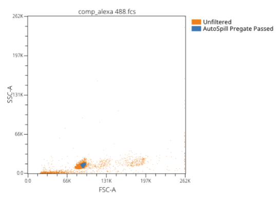
Autogating on Scatter Channels
An optional first stage of AutoSpill replaces the manual process of gating out contaminating events and debris. OMIQ determines the forward and side scatter measurement channels automatically and with some flexibility, with standard targets of “FSC-A” and “SSC-A”. After trimming extreme events at the margins, density estimation is used to determine peaks and perform Voronoi tessellation using the peak locations. The data contained in this tile is then used to obtain a rectangular subregion to repeat the process with a finer density estimation bandwidth. From the resultant tile, estimated density points exceeding a threshold value are determined and the convex hull of these points determines the polygon that is used as the final gate.

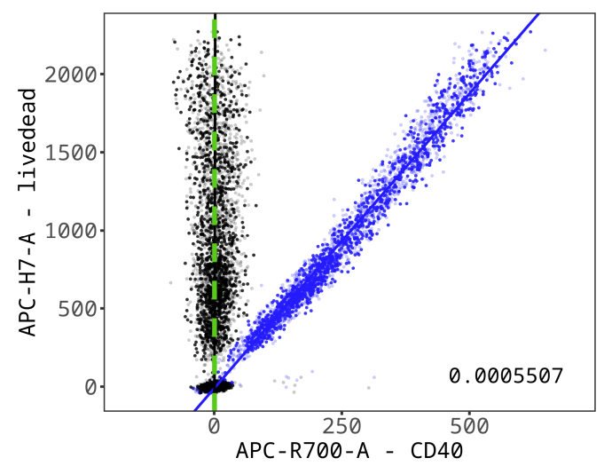
Calculation of Spillover Matrix
For each singly-stained control, the spillover from that dye into other channels is initially calculated as the slope of the robust linear regression of the measurements in the off-target channel versus the measurements in the dye’s target channel. The spillover coefficients on the diagonal (from the dye into its own target channel) are set to 1. This is essentially a direct extension of the approach of Bagwell and Adams, just substituting robust linear regression in place of measures of central tendency for discrete populations. This same general calculation is performed at each iteration of the optimization process.
Other Diagnostic Plots
For each singly-stained control, summary plots will be generated summarizing the corresponding coefficients from the spillover and compensation matrices.
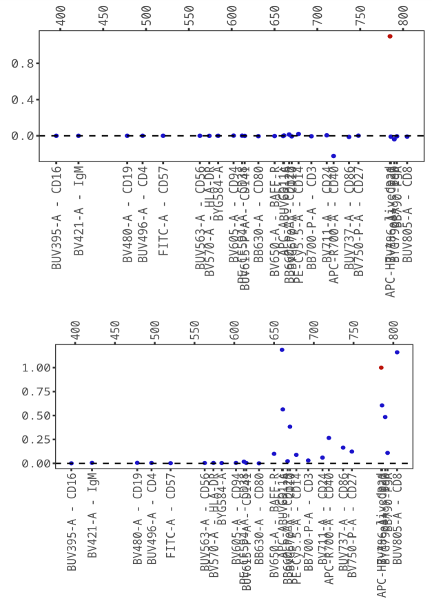
Intuitively, large spillover coefficients indicate large amounts of spectral overlap between dyes and channels. In OMIQ, similar information is presented in the heatmap of the compensation matrix within the Compensation task. For a direct measure of the quality of the compensation, AutoSpill provides density plots of the compensation errors from all pairs of channels. It also provides density plots of the skewness of the spillover values. In both cases, the density plots outlined by solid lines indicate positive errors or skewness while the dashed lines indicate negative errors or skewness. This allows for easy assessment of both the magnitude of the errors and whether they have a strong positive or negative bias. Large skewness values can be indicative of unhandled autofluorescence.

Additional Technical Notes
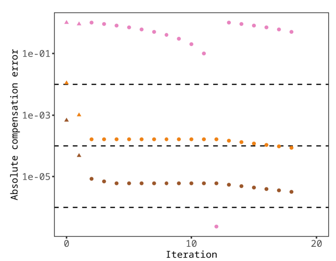
Refinement/Optimization of the Spillover Matrix
AutoSpill uses an iterative refinement step to optimize the spillover matrix. As a first step in refinement, the control files are compensated using the initial spillover matrix, but there will still be deviations from ideal compensation. Ideal compensation here is defined by linear independence of all channels after compensation, or equivalently an axis-aligned slope for all robust linear regressions of off-target channels for any given singly-stained control. As is laid out in the paper, it is possible to separate the errors in the spillover matrix and the errors in resulting compensation to enable iterative refinement to approach ideal compensation.
This is done very similarly to the initial calculation of the spillover coefficients, by obtaining robust linear regression models for each pair of channels. However, for off-target channels, nonzero slopes in this case represent errors in compensation that must be corrected. Theoretically, the errors in the compensated values should be equal to the negation of the product of the matrix of these errors and the true underlying spillover matrix, allowing for correction to the true spillover matrix. In practice with real data, an approximation of this true solution must be approached iteratively, which is precisely what AutoSpill does. It repeats this process of using the spillover matrix to calculate compensated values and determining the errors in the resulting compensation which allows improvement of the spillover matrix. It does this until the maximum compensation error is below a predetermined threshold.
Multiple Scaling
The AutoSpill refinement process assumes that data will ultimately be transformed using a biexponential transformation before analysis. Because of this, during the refinement process, once the error decreases below a certain threshold, it will switch to compensating and transforming the values before determining the compensation error. Currently, the implementation of AutoSpill in OMIQ does not do this. This is primarily due to the fact that OMIQ supports other transformations and so it does not necessarily make sense to optimize values under the assumption of a particular biexponential transformation. Further, internal testing has suggested this also does not appear to make a substantial difference to the quality of the compensation result in most use cases. It is possible in the future that support will be added for other transformations and the two-stage refinement process will be supported from the OMIQ implementation.
Recommended Resources
OMIQ Support Center
Find the answers to frequently asked questions or contact support.
Two Window Analysis in OMIQ
Learn how to access your workflow from two separate windows simultaneously.
Sharing, Collaboration and Groups
Learn how to share your datasets and workflows, set roles and permissions, and create groups.
How to Register an Account
Instructions on how to register your account so you can get started using OMIQ.
More OMIQ Resources

VIDEO SERIESGetting Started With OMIQ
Master the basics of OMIQ with this short video series covering the interface, metadata, feature names and the OMIQ workflow.

GUIDECytometry Analysis Tutorial
Get started with OMIQ using this in-depth tutorial that follows a complete end-to-end workflow.

VIDEO SERIESHow to Use Compensation
Discover how to manage compensation or calculate compensation from a single stain with this short video series.

GUIDEGuide to Using SAM in OMIQ
A guide to using the differential statistical analysis method SAM, available in OMIQ.
Experience the future of flow cytometry.