Cytometry Analysis Tutorial

Introduction

Thanks for your interest in OMIQ Data Science Platform!

This document is a mix of tutorial and documentation for using OMIQ for cytometry analysis. It can be followed linearly for a complete end-to-end workflow going from raw data to statistical significance, or you can search for specific topics.

If you do this tutorial you will be in very good shape for using OMIQ and for executing high-dimensional analysis workflows.

While our first priority is perfecting cytometry analysis, it should be noted that OMIQ is not specifically a cytometry analysis software. It is a data science platform meant to integrate all biomedical analytics (and more) eventually. This is what drives the design of our software, which is built around a flexible and simple “syntax” of stepwise operations on data. It is inspired by the needs for generalizability, data integration, and to promote auditable and reproducible analytics.

For these reasons, certain analytical goals for cytometry may be accomplished differently than you are used to with other cytometry-specific software. While most of the same things (and much more) are possible with OMIQ, you may have to take slightly different steps than you are used to, and to think differently about data analysis. We hope you see the ultimate benefits, not only for the sake of auditable, reproducible science, but for your own development of highly valuable data science skills.

OMIQ is improving all the time. Fluidity and flexibility, speed, available algorithms and visualizations, and everything else in the platform is evolving continuously. The most exciting and novel developments are yet to come. We hope to hear your feedback and requests so you can be part of the process!

Don’t forget that OMIQ is fully supported. Get in touch with us at any time by emailing support@omiq.ai

Enjoy, and don’t hesitate to get in touch.

– The OMIQ team

Visit the OMIQ Resources Center for more videos and guides.

Inspiration and High Level Overview

Want some ideas about what OMIQ can do? Watch this video:

In the video we demonstrate OMIQ platform principles and how to quickly go from raw data to p values while also interacting flexibly and deeply with data at the single-cell level. It is incomplete and meant just for inspiration.

This tutorial walks through a similar workflow step by step, exploring details along the way.

Step 1: Setup and Getting Started

Software Requirements

The only thing you need to use OMIQ is a web browser. Note that not all browsers are created equally, however! Chrome, Firefox and Edge should work best. Safari should mostly work. Avoid Internet Explorer. Regardless of browser, make sure you keep it up to date, not only for using OMIQ but because it is a best practice for security.

OMIQ is also supported on mobile devices to a certain extent. Smartphones and tablets can do in a pinch for viewing data and running tasks. Computers offer a better experience in general.

Disable Gesture Back Navigation

Many laptops and some external mice have a capability to navigate your browser forwards and backwards with a gesture. In practice, this produces mostly false positives and unwanted navigation. We strongly recommend you disable gesture navigation. This is important because we cannot effectively prevent your browser from navigating backwards and most (but not every) place in OMIQ has a safety mechanism to prevent you from losing progress in this case.

Browser Zoom

If you need to see more information in the OMIQ interface, zoom out. If you want to narrow in on something, zoom in.

Zooming out is done with the plus and minus keys on your keyboard in conjunction with the command (Mac) or control (PC) keys. The 0 key returns to default zoom level. There are other ways to control zoom within the View menu bar of the browser.

Take A Moment to Understand

OMIQ is different from most other cytometry software. It makes certain fundamental principles of analysis explicit to you, whereas normally you may be used to these being hidden or implicit.

It is built in a way that makes it powerful, but requires a bit more understanding of data analysis principles that are usually hidden by historical cytometry software.

Step 2: Understand the Vocab

The field of cytometry tends to use specific vocabulary that is confusing to outsiders, even those that are otherwise experts in data science. OMIQ uses traditional and widely accepted data science vocabulary (or reasonably close to it) to fit with broader standards. The list below translates common terms between cytometry-specific and traditional vocabulary.

Cytometrists can benefit from these translations to understand OMIQ better and to cultivate a better basis of communication with bioinformaticians and data scientists unfamiliar with Cytometry. The reverse is true of those individuals desiring a better understanding of cytometry vocabulary.

• An event is a row or observation. Sometimes called a datapoint.
• A channel or parameter or marker is a feature or column.
• A sample is a file. This is based on an FCS or CSV file on the disk of a computer that is uploaded to OMIQ.
  • It should be noted that sample is an ambiguous word because sometimes individual
    samples occur over multiple files.
• A gate may also be called a filter. A gate is just a specific type of filter and serves to subsample rows from a file or files.

Here are some fundamental OMIQ terms:

• A Dataset is a collection of files uploaded to OMIQ. A Dataset is like a folder for data.
• A Workflow is created inside a Dataset and is how analysis of data is carried out.
• A Task is an individual unit of analysis within a workflow. For example, scaling, compensation, gating, and t-SNE are tasks. Tasks are sometimes called jobs or algorithms in the cases where the task can be described in this way. The word plugin may also be used.
  • Note that OMIQ has a plugin system for installing any script as a custom task. Contact us if you’re interested in this!

Within certain documentation and videos we may use cytometry-specific vocabulary. We do this when the subject of explanation is cytometry-specific or the media is meant for a cytometry audience. Often we go back and forth between general and specific vocabulary in these cases as well.

Step 3: Download the Tutorial Dataset

Zip of files: https://omiq.ai/docs/files/OMIQ-tutorial-files.zip

Note the browser may indicate a problem previewing the file. That’s okay, you just need to download it.

Note the files are FCS files that were converted to CSV. You can think of them as FCS files. If you prefer FCS, an FCS version is available here: https://www.omiq.ai/docs/files/OMIQ-tutorial-files-FCS.zip

However, note that the FCS version does not have feature names that need to be corrected. You can simply skip that part of the tutorial or still experiment with changing feature names as desired.

Download the file and unzip it to reveal the CSV files inside. These individual files are what we will upload to OMIQ. Note that the zip cannot currently be uploaded as a single file.

The Dataset is an abridged and cleaned-up version of Hartmann et al 2019 mass cytometry Dataset (http://flowrepository.org/id/FR-FCM-Z244). The files are GVHD patients at 30 days and 90 days post bone marrow transplantation. The tissue is PBMC.

► Watch the Getting Started video series

Step 4: Create a Dataset and Upload Data

Create a Dataset in OMIQ and upload the files. This is fairly simple and thus won’t be demonstrated here.

All files uploaded to OMIQ must be inside of a Dataset.

Files can be CSV or FCS. Note that multiple files grouped together in a ZIP file is not currently supported. However, if uploading CSV files, individual files can be zipped to save space. To be clear, if a zip file is ever uploaded to OMIQ, it must only contain a single CSV file inside it. Support for multiple files within the same zip will be added in the future.

Files can be analyzed as soon as they are done processing. Processing status can be monitored from the page where files are uploaded. Note that it is not necessary for all files to be completed uploading or processing before analysis can begin. They will continue to upload in the background as you do other actions.

Files can be deleted by clicking the filename from the list of files. Inside the details page for that file there is a delete button which can be clicked to remove the file from the Dataset permanently. Files can also be deleted in batch from the dataset main page.

Consider reviewing the section on Folders and Tags.

Step 5: Set Metadata and Edit File Names

An important first step in order to fully leverage OMIQ is to assign metadata values to your files. Metadata are tags of information associated with each file in a Dataset that provide experimental or clinical context. Metadata can be continuous or categorical. These metadata go on to power a variety of functionalities within OMIQ.

File names can also be edited directly within OMIQ. This is discussed in the video overview. To edit filenames, use the spreadsheet editing strategy, modify the names, and then paste them into OMIQ, making sure to include the OmiqID column. If you are only editing file names without adding metadata, you will need to visualize the changed names in the Files tab since the metadata tab will be empty.

You can also import metadata from FCS files:

Notes

• Editing this information does not alter the underlying raw data. Raw data are never altered within OMIQ. All operations on data are stored as “layers” on top of the raw data.

Step 6: Review and Edit Feature (Channel) Names

A tragic problem that can befall a cytometry experiment is having different feature names across different FCS files. This can prevent proper analysis and be very hard to correct. However, with OMIQ, this can be solved easily!

Sometimes you may have missing, extra, or misordered features between files. This can result in OMIQ highlighting what appears to be a conflict in names between files, but in reality is just an ordering issue and is ultimately harmless. If this is the case, just ignore it. All OMIQ functionality will still work fine. Don’t try to correct the order. Features have a given order that cannot currently be changed. Please watch video for an explanation of these concepts.

Notes

• If there are disagreements between files on the primary feature name, the worst case scenario is not being able to choose that feature for certain forms of analysis on groups of files. This is because in a grouped analysis, only features shared by all files may be selected.
• If there are disagreements between files on the secondary feature name, the correct value will be chosen depending on which file is selected or being viewed, or in the case of grouped analysis, all names will be displayed in a comma-separated list.
• Editing this information does not alter the underlying raw data. Raw data are never altered within OMIQ. All operations on data are stored as “layers” on top of the raw data.
  

Step 7: Start a Workflow

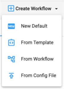
Now that the Dataset has been configured, click this button to start a new workflow (choose New Default):

All analysis in OMIQ is done within workflows. A workflow has access to the data within the Dataset. All filenames, metadata, and feature names will be present in all workflows in the same state they are within the Dataset.

OMIQ will make its best effort to start the workflow for you by initializing compensation and scales as relevant if you are working with cytometry data.

Whether or not you know it, any software you have used for cytometry analysis applies analytical steps to your data automatically and in a particular order. It’s implicit and somewhat hidden. In OMIQ we make all operations on data completely clear in their nature and ordering.

In Cytometry, the classical steps to apply are compensation and scaling, in that order. Where compensation is not applicable, scaling is applied only. These steps and more are described below.

Sidebar: Compensation

This is not properly part of the tutorial but is discussed here anyway.

Overview of managing compensation(s)

This overview covers various considerations for adding and editing compensation.

Notes

• Scales must also be set in order to properly visualize the effect of the compensation. The video demonstrates this. See the data scaling section for more details about data scaling.
• Compensation will be applied automatically if it is detected within the FCS files. It can also be
  applied by the arbitrary creation of compensation matrices and their application to groups of files.
• Compensation matrices can be edited directly by clicking and editing certain values. Alternatively, a matrix can be copied from a spreadsheet and pasted into OMIQ, overwriting the existing matrix that is currently selected.
• To copy a compensation matrix out of OMIQ, just click the appropriate button. Then paste it into a spreadsheet or on top of another comp matrix in OMIQ.

Calculating compensation from single stain (single color) control files

This overview covers the creation of compensation matrices from single stain control files.

Remember the structure of the Workflow is nuanced and important when calculating compensation. One branch must be created without compensation (but with scaling) in order to create the matrix. Then the created matrix is used in the other branch with compensation in order to apply it in typical Workflow context.

• The first branch is root → scaling → create comp
• The other branch is root → compensation → scaling → …
  • You put the created compensation in the underlined comp task in the second branch.

The AutoSpill Algorithm

AutoSpill is a modern and innovative algorithm for calculating compensation matrices from single stain controls and an alternative to the traditional method detailed above.

See the special AutoSpill documentation and guide

► Watch the AutoSpill video series

Step 8: Adjust Scaling / Transformation

In our experience, data scaling (aka “transformation”) is perhaps the most poorly understood part of analyzing cytometry data. This is unfortunate because the application of scaling equations and their particular settings have a significant effect on data analysis results and reproducibility. This is especially the case when using machine learning techniques.

Notes

• Contrary to the video, OMIQ now automatically configures your scale settings. As is
  industry-standard, we do this by heuristic by looking at the instrument of origin.
• Scale settings may need to be adjusted if the heuristic settings are not appropriate. This is
  uncommon for mass cytometry data but fairly common for fluorescent cytometry data. The critical setting is the cofactor for arcsinh scales. Increase it to compress the region around 0. Decrease it to expand the region around 0. The correlate setting for biexponential scales is the width basis. Note that biex scales are not currently supported in OMIQ but arcsinh is similar (and simpler). For more info, see the deep dive document below.
• Scale settings can be copied and pasted between tasks.
• Unless you know otherwise, you almost certainly should not use the Log10 scale type.

Deep Dive Into Scales and Relation to Numerics Properties of Data

Want to deepen your knowledge on this fun topic? Check out this article.

Scaling is generally the most poorly understood (yet extremely important) element of cytometry analysis. We strongly recommend an understanding of this subject and we consider it essential for anyone using cytometry as a core technology in their research!

Sidebar: Set Display Boundaries for Plots

This is not properly part of the tutorial but is discussed here anyway.

Display boundaries are the minimum and maximum for data display on plots. These boundaries are tracked within the workflow and can be changed anytime a plot is visible. OMIQ will try to set yours automatically, however, you may need to adjust them. Watch the video to learn the efficient way of doing this in bulk.

Step 9: Do Cleanup Gating

At this stage of analysis, it's likely that cleanup gating would be needed.

Remember that you can set gates in a specific position per file, for example, to deal with batch variance:

OMIQ has all boolean gate types (AND, OR, NOT), however they are called boolean filters. To create a boolean filter, right click the filter within the filter tree and select the desired boolean option.

One question about boolean filters that sometimes comes up is how to make boolean filters between disconnected positions in the gating tree. Watch video for an explanation of this situation and how to accomplish that goal.

Notes

• The example data for this tutorial has already been cleaned. Thus, this step isn’t technically necessary but it’s useful to illustrate it anyway. Note also that this gating task will be used to insert gates into the workflow later on in the tutorial.

Step 10: Subsample your Data

When you have gated your data it doesn’t mean you have made any particular choice about applying a gate to your data. It simply means those gates are available within the workflow from that point onward.

Actually filtering the data down by some gate or filter, or simply downsampling the number of rows, is fulfilled by the Subsampling task.

This design is meant for convenience to avoid setting downsampling settings redundantly, for example, when doing numerous runs of an algorithm.

Notes

• The subsampling in the example video is pointless because our gate and count setting results in no actual sampling of the data. It’s simply done for demonstration and discussion purposes.

Step 11: Run Dimension Reduction

At this point the workflow can go many different directions based on specific needs. The following steps are merely suggestions based on common operations.

Most workflows these days use some form of dimension reduction. Thus we will start there. We will run opt-SNE but the principles of setup and analysis apply to all dimension reduction algorithms.

Notes

• The UMAP that appears in this video does not appear in the rest of the demo for simplicity.
• Do not concatenate data prior to running any algorithms in OMIQ. The system takes care of this automatically behind the scenes and separates the data back out again for downstream analysis. Make sure to learn about virtual concatenation for downstream analysis.
  

Side Note: Task Computational Limits

Tasks (aka “algorithms”, “plugins”) have a certain amount of CPU and memory allocated to them by default. Depending on the size of your Dataset and the parameters of the algorithm you are using, the allocated amount of CPU and memory may not be enough. This can result in execution failures. If this happens, feel free to get in touch with support@omiq.ai to understand what happened, find alternative algorithms or algorithm settings, or to increase the computational power allocated to the task.

Step 12: Dimension Reduction Results Visualization

Regardless of the dimension reduction algorithm used there are common operations for interpreting the results. The result of a dimension reduction is usually termed a map or embedding.

Here we will overview some common operations for analyzing and comparing embeddings.

Sidebar: Gating and Exploring an Embedding

Note: this is just a sidebar for people interested in gating t-SNE maps or correlating the t-SNE map to the low-dimensional data. The results are not taken forward into the rest of the tutorial. However, this section is valuable to consider and understand.

Step 13: Clustering (with Metaclustering)

Clustering is a common operation for categorizing single-cell data into ostensible cellular populations. Later, these populations will be analyzed for differential signatures between the patient groups.

We use FlowSOM with metaclustering in this tutorial. However, any other clustering algorithm could be used instead. The principles are the same, it’s just the algorithm producing the clusters that is different.

Discussion: Does Task Order Matter?

To follow up on the end of the previous video, here is a common question that leads to good discussion:

Why, in our tutorial, does clustering come after dimension reduction? Does one have to come before the other? The answer in this particular case is: there is no reason. It’s an arbitrary decision. The order could be swapped without issue. That is because in this case we are not clustering the output of the opt-SNE task. We are clustering the original data only.

However, there is a scenario in which we might want to cluster the 2 resulting columns from the opt-SNE task. Clustering a dimension reduction map is an oft-debated practice that nonetheless is fairly common. If this were our goal, then we would be forced to run FlowSOM after opt-SNE, such that the opt-SNE columns would be available for the FlowSOM algorithm to cluster them.

In both cases discussed above, the workflow tree would appear the same. It is a good example to show that the structure of the workflow tree does not always tell you exactly what is happening to the data flowing through it. To know for certain, you need to open the task and look at its settings. The structure of the workflow is more flexible; it can also simply represent an accumulation of results. The order may matter in the case of dependent operations, or it may not, in the case of independent operations. The only consideration is that if you want to use both results at the same time, such as in the figures we are about to make below, they must be in the same “lineage” of tasks within the tree.

Step 14: Convert Cluster Results to Filters

By default, clusters (or metaclusters, which are just another form of cluster) are stored as new columns of data. Each row in the column is given an integer ID (e.g., 1, 2, 3, 4…) to indicate which cluster it is a member of.

In order to continue doing useful analysis, we need to convert these numerical results into filters that represent each cluster. Another term sometimes used for this is “cluster gates”. Once the clusters are converted to filters, we can make plots, heatmaps, export stats, and otherwise quantify them in many different ways.

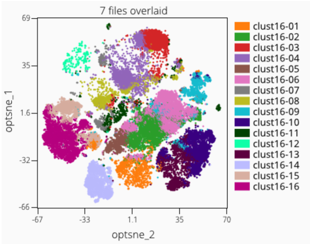
Step 15: Cluster Overlays

It is a common operation to want to overlay clusters on an embedding. This is used to understand if the clustering and dimension reduction are reasonably concordant in finding patterns within the high-dimensional data, and can also help understand if the data may be over or under clustered.

Step 15.1: Splitting and Merging Clusters

An operation of interest that relates to the visualization of clusters on a dimension reduction map is to either split or merge certain clusters.

Step 16: Export Statistics

OMIQ can export CSV files of batch statistics. Want a statistic that we don’t have? Let us know!

Step 17: Clustered Heatmap

Another way to understand the feature characteristics or abundance patterns of each cluster is to use a clustered heatmap.

Clustered Heatmap

Step 18: Locks and Adding Gates

Locks are designed to protect the dependencies within a workflow. However, sometimes they can be validly overridden. Here we discuss the concept of locks and how to unlock certain tasks to edit them. We also insert a gate that we will use in the next step.

Notes

• In this video we only insert a new CD3+ gate. To participate fully in the next step you may consider adding more similar single-positive gates.
• Be very careful when overriding locks. They are there for your protection! Serious problems can emerge from modifying something in your workflow that the downstream depends on.

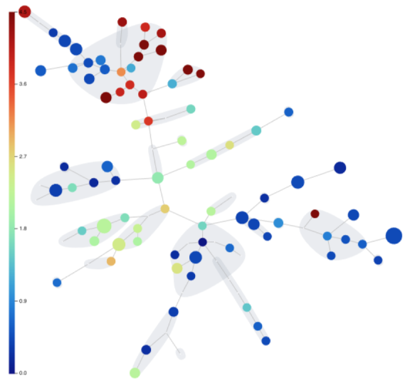
Step 19: Graph Analysis and Graph Filters

This step isn’t strictly necessary to complete the tutorial but it can still be participated in.

One of the results that our FlowSOM produced is a minimum spanning tree of clusters. A tree is a form of graph. Any graph produced by any algorithm in OMIQ can be analyzed using the Graph Viewer. This is a powerful analytical interface that provides data exploration and filtering functionalities.

Step 20: Statistical Differential Analysis & Volcano Plots

What are the most interesting differences between patient groups within our Dataset? What is the statistical significance of these differences? OMIQ has methods to help answer these questions. In this case we will demonstrate the edgeR method to test for differential abundance between our day 30 and day 90 patient cohorts and visualize the results on a volcano plot.

Step 21: Box and Violin Plots

Box and violin plots are an excellent way to visualize differences across a dataset. This visualization automatically links to file metadata for a simple configuration process.

Box and violin plots

When viewing a box plot looking at feature data (with a metric of mean, median, etc.), you may notice a difference in units compared to typical OMIQ plots:

In the example above we are viewing the same information (though at different levels of detail) between box plots and histogram overlays. The units on the axes have been called out as the typical point of confusion because they are different between the plots but one would expect them to be the same.

To understand this difference fully, you should read our article on understanding data scaling.

In brief, cytometry software classically uses a labeling trick on plots to display the units in the data’s original range. These are usually larger values (as in the histogram overlay). In reality, the underlying data are actually in different numeric units as a result of the critical workflow step of data scaling. Scaled values are much smaller as a consequence of a log-like transformation.

The box plot is showing the true values. The histogram is drawn using the true values but the axis labels use a trick to reverse the real values back to the original range. This is often called reverse transformation or inverse transformation. We anticipate adding this labeling trick to box plots in OMIQ at some point also. If you require it now for some reason, remember you can easily calculate the reversal yourself and change the labels outside of OMIQ. We have included a reversal spreadsheet formula in the aforementioned article on understanding data scaling.

Step 22: Exporting Plots and Figures

Exporting plots and figures in OMIQ is done in different ways and in different available formats depending on the type of plot. Examples include PNG, SVG, PDF, PPT (PowerPoint), etc. In general you will either be grabbing one plot at a time or exporting them in batches from an OMIQ Figure.

Individual Plots

Exporting individual plots usually involves finding a button on or near the plot to export it. Alternatively you may have to right-click the plot to see options to copy it for pasting into a different software or to download the image. Watch the video overview of getting individual plots out of OMIQ. Note the video says Figures cannot currently be exported in a batch format but that is no longer correct information (read below).

Exporting OMIQ Figures

There are two general ways to export a Figure:

1. Exporting the Figure with the plots as they are currently. This is an intuitive option to take
   everything you see on the page and package it up for export.
2. Exporting a batch report with the Figure as a batch template. The batch report will take the
   template of the figure but analyze one file at a time from the Dataset within the template. What results is a potentially large combined set of individual figures where each figure is for one file.

Format can also be chosen as part of the export process. As of the time of writing, Figures can be exported as PDF and PPT.

OMIQ Fonts for PowerPoint Export

Fonts cannot be automatically embedded in a PPT file. Thus, when exporting to PPT, make sure to install the OMIQ font pack if you want fonts to look as they do in OMIQ. To do this, first download the font files from this link. The fonts are a small subset of Google’s open-source Noto Sans font. Once you’ve downloaded the fonts, follow the simple instructions from Google on how to install them for your operating system. However, omit step 1 because you have already downloaded the fonts from OMIQ.

Conclusion and Next Steps

Congratulations! You’ve gotten through the tutorial. You’ve learned quite a bit and should understand how to go forward from here with your own data.

You should think of the tutorial we did with the workflow as being fairly generic. Different methods can be swapped in for similar effect. For example, for clustering you could use Phenograph instead of FlowSOM + metaclustering. You could even use manual gates instead of clustering. You could use EmbedSOM for dimension reduction instead of opt-SNE. You could use SAM for differential analysis instead of edgeR.

The workflow demonstrated here is a series of conceptual steps that can be accomplished with different methods. Which methods confer advantages or disadvantages in certain situations is something we can help you understand or that you can learn on your own with our documentation. Or you can experiment with them yourself. Curious to try some methods that aren’t in OMIQ? Let us know!

Get support at anytime by emailing support@omiq.ai

Miscellaneous Topics

Miscellaneous topics are covered below with instructional videos and pointers.

Folder and Tags

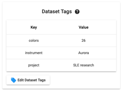
A question that comes up every so often is whether or not OMIQ has folders (like those found on a traditional computer system) to help organize datasets. The current answer is no. We are considering implementing this functionality, though we have an alternative that we feel is better. It is a search functionality using Dataset Tags.

Dataset Tags are metadata associated with a Dataset. The concept is similar to metadata associated with files. You administer Tags from inside of a Dataset using the Tag manager widget (example below). Tags can also be set in bulk from the Datasets list page.

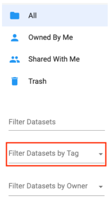
From the Datasets list you can use the indicated selector below to filter Datasets by Tags. Note that you can choose multiple tags at once (which broadens the search as an OR operator).

Gating Hierarchy Plots

Sometimes you need to quickly see the sequence of gating steps for a given population. You may also want to see the gating hierarchy for all files in a Dataset. This can be done easily in the figure.

SAM

SAM is a differential statistical analysis method. It finds the most significant stratifying signatures between files organized by metadata. It reports these differences as differences in abundance of cellular populations or signaling differences of chosen markers within these populations.

► READ SAM OVERVIEW GUIDE

► Watch the video series of Statistical Differential Analysis

Interactive Gating

Project gating choices “backwards” or arbitrarily onto plots of your choice.

Concatenation

Files can be concatenated in OMIQ in two ways. The first is “virtual” and the second is “permanent”.

Virtual concatenation is a convenient functionality that allows files to be concatenated dynamically during plot generation.

Permanent concatenation creates a new file within OMIQ. This should only be used when it’s required to reconstitute a sample that was acquired over multiple FCS files due to length of acquisition. This is common when working with CyTOF data.

NOTE: Permanent concat should not be used prior to running an algorithm. All algorithms in OMIQ automatically concatenate your data during execution and separate it out again for analysis. Furthermore, permanent concat should not be used for visualizing data. Use virtual concat instead. Lastly, remember that heatmaps have their own concat setting within the task.

Trajectory Analysis

OMIQ currently has two trajectory analysis algorithms, Wanderlust and Wishbone. The separate guide below is highly recommended (likely even required) reading for anyone trying to do these types of analysis.

► WANDERLUST AND WISHBONE GUIDE

► Watch the video series on Trajectory Interference

flowAI

flowAI is an algorithm for automated data cleaning. The standalone flowAI guide below also covers principles applicable to any other cleaning algorithm in OMIQ (e.g., flowCut, PeacoQC), especially with respect to the concept of the pre-filter and interpretation of results.

► FLOWAI GUIDE

► Watch the video series on Automated Data Cleaning

flowCut

flowCut is an algorithm for automated data cleaning. The algorithm’s general documentation (written by its authors) is available below and is quite detailed about the algorithm and its settings. Remember to also consult the flowAI and general cleaning guide above in order to learn general principles about running any cleaning algorithm in OMIQ, such as viewing results.

► FLOWCUT SETTINGS GUIDE

PeacoQC

PeacoQC is an algorithm for automated data cleaning. An OMIQ guide is in development. Between the paper, online resources, and the flowAI and general cleaning guide above, you should be successful with PeacoQC.

Sharing, Collaboration, and Groups

There’s no need to be lonely on OMIQ!

Forming Connections

Before you can share anything, you must connect with other users. To do this, go to your profile page and enter in email addresses of other OMIQ users. They will get a notification about your connection request. When they accept you will be able to share with them.

Sharing Datasets

A Dataset can be shared from the collaborators tab in the Dataset.

Keep in mind that when you share the Dataset it does not mean the user will have access to all the workflows. Users must be specifically added to workflows for them to get access.

Sharing Workflows

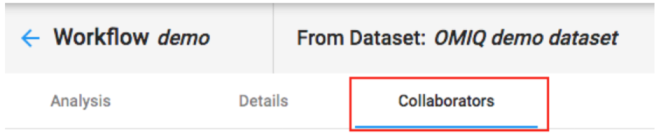
A workflow can be shared from the collaborators tab in the workflow.

When a user is added to a workflow it will automatically give them reader access to the Dataset. So, in most cases, a user should just be added directly to a workflow and not to the Dataset prior, since that part is automated. The exception is when they need a higher access level on the Dataset.

Roles & Permissions

A user added to a Dataset or workflow can be a Reader or Editor. Give someone reader access to limit their ability to edit the resource. Editor access, as the name implies, means the user can edit the resource.

Groups

On your profile page, underneath the Connections pane, there is a Groups pane. Here is where you can create and manage Groups. A Group is a collection of users that work together or otherwise share access to certain Datasets and Workflows. Instead of sharing with individual users, you can share with the Group to give all the users in the Group access to the resource. This is generally easier and less prone to error. Furthermore, new users can simply be added to the Group in order to give them access to all the underlying resources the Group has access to, or conversely removed upon leaving the Group. This is much simpler than adding or removing individual access for many resources individually and separately.

In order to add users to the Group, you must be connected with that user. The exception to this rule is for user administrators, a special role for OMIQ enterprise clients.

If a user has direct access to a resource in addition to Group access to a resource, but different roles in each, they will get the greatest role from among their multiple means of access.

Changing Owner of Resources

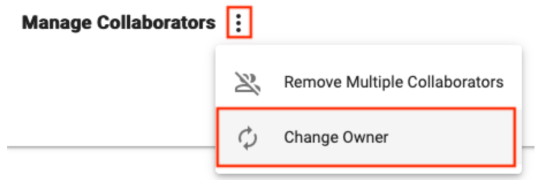
Related to Sharing and Collaboration, it may be necessary at some point to change the Owner of a resource. Currently, any resource can only have one Owner, and being an Owner confers special privileges, such as the ability to delete the resource.

Look for the Change Owner button in the extra actions menu within the Collaborators pane of a resource to change the Owner, which can be a Group or individual user.

Ownership can also be changed in bulk. This is a common strategy when leaving a research group and needing to transfer ownership of all assets to someone else. In this case our recommendation is to transfer ownership to a Group with one or more responsible colleagues as members. That way access can easily be passed on again as necessary by adding people to the Group. Follow these instructions to bulk transfer:

1. Make sure your account has formed a connection with the receiver account.
2. In your account, go to the Datasets list page, filter to those Owned By You, and open the menu in the top right to reveal the option to Bulk Change Owner.
3. Do the same thing from the Workflows list page to also transfer the Workflows you own. Remember these are separately managed from Datasets.

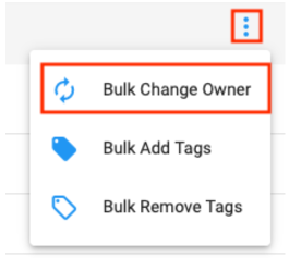
Note: consider using Bulk Add Tags for Datasets before transferring ownership in order to tag a piece of useful information such as you being the original owner.

If your account email is registered as the billing contact, remember to email billing@omiq.ai to transfer this responsibility to the new account!

If a user leaves before bulk transferring, OMIQ staff can initiate the transfer with admin powers.

OMIQ Resources

• OMIQ Resources Center
• Understanding Data Scaling
• SAM Overview
• Autospill Algorithm
• Trajectory Analysis (Wanderlust, Wishbone)
• flowAI and Cleaning Algorithms
• Support Center